The First Order Greeks
The option greeks are used describe the different dimensions of risk involved in taking an options position in the market. These dimensions are referred to as the option greeks because they are represented by greek symbols. In plain english, the greeks describe how the option price changes when each of the parameters are changed (holding all others constant).
\[\Delta = \frac{\partial V}{\partial S}, \hspace{0.5cm} \theta = \frac{\partial V}{\partial \tau}, \hspace{0.5cm} \nu = \frac{\partial V}{\partial \sigma}, \hspace{0.5cm} \rho = \frac{\partial V}{\partial r}\]The purpose of this article is explore the first order greeks for a European call and put option where the underlying does not pay dividends. This article also demonstrates a simple implementation framework using Python.
Black-Scholes Equation
The Black-Scholes model is a partial differential equation (PDE) which is a multivariate function that explains the value of an option given changes in other intrinsic and market parameters. The Greeks are simply the sensitivity of the PDE to changes in the parameters. Many PDE are difficult to solve or are computationally expensive, however, the Black-Scholes model has been thoroughly researched and there are known closed for solution which reduce the computation expense to compute these metrics.
The Black-Scholes equation is used to value options based on a no arbitrage argument. The Black-Scholes equation takes the form
\[\frac{\partial V}{\partial t} + \frac{1}{2}\sigma^2 S^2 \frac{\partial^2 V}{\partial S^2} + rS \frac{\partial V}{\partial S} - rV = 0\]Gradient
In mathematics, the partial derivatives of a PDE are referred to as the gradient \(\nabla\) of the function. Consider the function with \(n\) parameters
\[f(x_1, x_2, \dots, x_n)\]The gradient of this function would therefore be
\[\nabla f(x_1, x_2, \dots, x_n) = \Bigg \langle \frac{\partial f}{\partial x_1}, \frac{\partial f}{\partial x_2}, \dots, \frac{\partial f}{\partial x_n} \Bigg \rangle\]Within the Black-Scholes model, there are four parameters which can be determined from the gradient using closed form solution for European Call and Put option. However, exotic options don’t always have closed form solutions and therefore differential solvers may be required which are often computationally expensive.
The Greeks
The four variables in the Black-Scholes model are as follows. The value of the derivative (call/put) is represented by \(V\).
- Delta - \(\Delta\) - First partial derivative of the option value w.r.t the asset price \(\frac{\partial V}{\partial S}\)
- Theta - \(\theta\) - First partial derivative of the option value w.r.t time \(-\frac{\partial V}{\partial \tau}\)
- Vega - \(\nu\) - First partial derivative of the option value w.r.t the asset volatility \(\frac{\partial V}{\partial \sigma}\)
- Rho - \(\rho\) - First partial derivative of the option value w.r.t the interest rate \(\frac{\partial V}{\partial r}\)
European Option Greeks
The value of a European call options can be derived from the Black-Scholes equation given a set of boundary conditions for the European option. The value of a call option is shown below.
\[C_t(S_t,t) = S_t N(d_1) - Xe^{-r(T-t)}N(d_2)\]Where
\[d_{1,2} = \frac{ \ln{ \left(\frac{S_t}{X}\right) } + \left( r \pm \frac{\sigma^2}{2}\right)(T-t)}{\sigma\sqrt{(T-t)}}\]- \(N(\cdot)\) - is the cumulative standard normal distribution
- \(T\) - is the time to maturity
- \(S_t\) - is the spot price of the underlying asset at time \(t\)
- \(X\) - is the strike price
- \(r\) - is the risk free interest rate
- \(\sigma\) - is the volatility of the underlying asset returns
The value of the European put option can be derived using put-call parity as
\[P_t(S_t,t) = Xe^{-rT}N(-d_2) - S_tN(-d_1)\]The closed form solutions for the first order greeks for the European call and put options are summarised in the table bellow
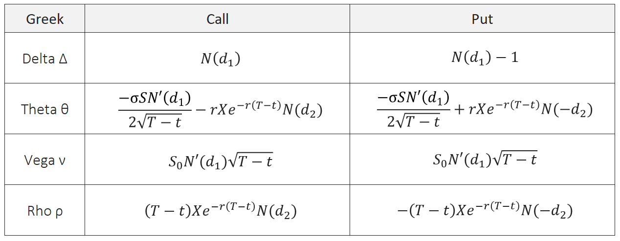
Summary of the Greeks for a European Option
Python Implementation
The implementation of the first order greeks for a European call option is shown below. The same can be done for a European put option.
import math
import scipy.stats as sp

class EuropeanCall:

    ''' Inputs
    S: Stock Price
    v: Volatility
    X: Strike Price
    T: Time to maturity
    r: Risk free interest rate
    '''

    def __init__(self, S, v, X, T, r):
        self.S = S
        self.v = v
        self.X = X
        self.T = T
        self.r = r
        self.price = self.call_price(S, v, X, T, r)
        self.delta = self.call_delta(S, v, X, T, r)
        self.theta = self.call_theta(S, v, X, T, r)
        self.vega = self.call_vega(S, v, X, T, r)
        self.rho = self.call_rho(S, v, X, T, r)

    def call_price(self, S, v, X, T, r):
        b = math.exp(-r * T)
        d1 = (math.log(S / X) + (r + 0.5 * v**2) * T) / (v * math.sqrt(T))
        d2 = (math.log(S / X) + (r - 0.5 * v**2) * T) / (v * math.sqrt(T))
        N_d1 = sp.norm.cdf(d1)
        N_d2 = sp.norm.cdf(d2)
        x1 = S * N_d1
        x2 = X * b * N_d2
        return x1 - x2

    def call_delta(self, S, v, X, T, r):
        b = math.exp(-r * T)
        d1 = (math.log(S / X) + (r + 0.5 * v**2) * T) / (v * math.sqrt(T))
        N_d1 = sp.norm.cdf(d1)
        return N_d1

    def call_theta(self, S, v, X, T, r):
        b = math.exp(-r * T)
        d1 = (math.log(S / X) + (r + 0.5 * v**2) * T) / (v * math.sqrt(T))
        d2 = (math.log(S / X) + (r - 0.5 * v**2) * T) / (v * math.sqrt(T))
        N_d1 = sp.norm.cdf(d1)
        N_d2 = sp.norm.cdf(d2)
        dN_d1 = math.exp((-d1**2) / 2) / math.sqrt(2 * math.pi)
        x1 = (S * dN_d1 * v) / (2 * math.sqrt(T))
        x2 = r * X * math.exp(-r * T) * N_d2
        return -(-x1 - x2)

    def call_vega(self, S, v, X, T, r):
        b = math.exp(-r * T)
        d1 = (math.log(S / X) + (r + 0.5 * v**2) * T) / (v * math.sqrt(T))
        N_d1 = sp.norm.cdf(d1)
        dN_d1 = math.exp((-d1**2) / 2) / math.sqrt(2 * math.pi)
        x1 = S * dN_d1 * math.sqrt(T)
        return x1

    def call_rho(self, S, v, X, T, r):
        b = exp(-r * T)
        d1 = (math.log(S / X) + (r + 0.5 * v**2) * T) / (v * math.sqrt(T))
        d2 = (math.log(S / X) + (r - 0.5 * v**2) * T) / (v * math.sqrt(T))
        N_d1 = sp.norm.cdf(d1)
        N_d2 = sp.norm.cdf(d2)
        x1 = X * T * math.exp(-r * T) * N_d2
        return x1
We can then calculate the first order greeks for a European Call.
price = EuropeanCall(S=100, v=0.5, X=150, T=20, r=.01).price
delta = EuropeanCall(S=100, v=0.5, X=150, T=20, r=.01).delta
theta = EuropeanCall(S=100, v=0.5, X=150, T=20, r=.01).theta
vega = EuropeanCall(S=100, v=0.5, X=150, T=20, r=.01).vega
rho = EuropeanCall(S=100, v=0.5, X=150, T=20, r=.01).rho
The output results are
- Price = 70.862
- Delta = 0.847
- Theta = 1.456
- Vega = 105.383
- Rho = 277.929
Summary
This articles has shown that the gradient of the Black-Scholes equation are the first order greeks, namely Delta, Theta, Vega and Rho. We have shown that the closed form solutions exist for the first order greeks of a European call/put options and demonstrated an implementation of these greeks in Python.