Gaussian Copula Simulation

A Copula is a multivariate cumulative distribution function which describe the dependence between random distributions. Copulas are often used in quantitative finance to model the tail-risk or returns of a set of correlated distributions (Marginal Distributions). There are many types of Copula which all have different application. The purpose of this article is to demonstrate how to simulate from a Gaussian Copula and the underlying mathematics.

Marginal Distribution

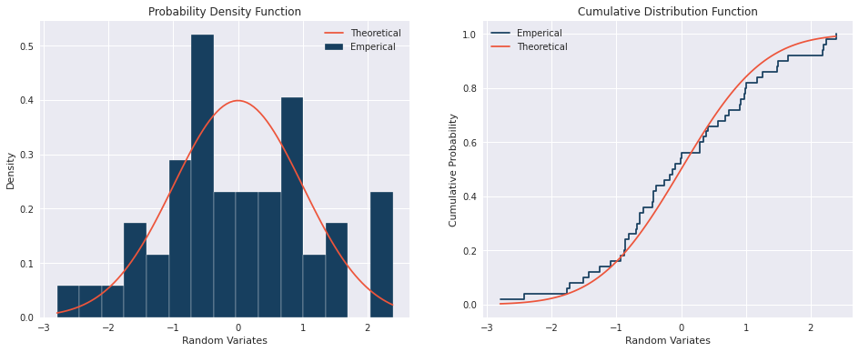
Consider a distribution \(X\) which we can simulate \(n\) random variates {\(x_1, x_2, \dots, x_n\)}. Each of these random variates are independent and identically distributed since they come from the same distribution and are mutually independent. We can refer to this as the marginal distribution \(f_X(x)\).

The charts below show an example of a PDF and CDF for an standard normal distribution with a sample size of \(50\):

Joint Distribution and Copulas

A joint distribution is a multi-dimensional distribution consisting of two or more marginal distributions which may or may not be dependent of each other. Sklar’s theorem states that every multivariate cumulative density function of random vectors \(X_1, X_2, \dots, X_d\) can be expressed in terms of its marginal distributions \(f_{X_1}(x_1),\dots,f_{X_d}(x_d)\). Therefore the join distribution is

where \(C\) is the Copula.

Simulating a Joint Distribution

Within in this section we will simulate the joint distribution for two different scenarios:

1. Independent marginal distributions - without using copulas
2. dependent marginal distributions - using a Gaussian copula

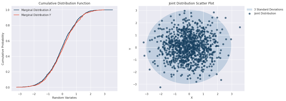
1. Independent Margin Distributions

In the case where the marginal distributions are independent, the joint distribution is known through the property of independence

By simulating from two independent standard normal distributions \(X\) and \(Y\), we can construct an empirical joint distribution as shown below. The mean and variance of the joint distribution is \(\mu = (0,0)\) and \(\sigma^2 = 1\).

2. Dependent Margin Distributions

The second case we will consider is when the marginal distributions are not independent, i.e. correlation exists between them. In order to account for the correlation between the marginal distribution, we will need to consider a copula.

The choice of copula is very important when considering more complex distribution. In this example we will assume standard normal marginal distribution with no particular interest in the tails of the distributions. If the marginal distributions were fat-tailed distributions (such as a Pareto distribution), then other types of copulas such as a t-copula may be more suitable. Particularly when we are interesting in tail events. Simulating from a t-copula will be explored in another article.

Let us define the correlation between marginal distributions as shown below. For this example we can also assume that the correlation is Pearson’s correlation.

Consider the example where we have two standard normal marginal distributions \(X\) and \(Y\) which are dependent. In order to determine the joint distribution \(f_{X,Y}(x,y,\rho)\) we need to simulate the variates of \(Y\), while taking into account the information already obtained from our simulation of \(X\).

Conditional Expected Value:

The expected value of \(y_1\) given that we know \(x_1\) is

\begin{equation} \notag E(y_1|X=x_1) = \mu_Y + \underbrace{\rho \cdot \sigma_Y \cdot \left( \frac{x_1 - \mu_X}{\sigma_X} \right)}_{\text{Scaled Mean Shock}} \end{equation}

This equation is basically saying that the expected value of \(y_1\) given that we know \(x_1\) is the original mean of \(Y\) plus a shock to account for the fact that \(x_1\) may be different than the original mean of \(X\). Note that in the event that \(x_1=\mu_X\) then the expectected value of \(y_1\) would be the original mean of \(Y\) which is \(\mu_Y\).

Conditional Standard Deviation:

The standard deviation of \(y_1\) given that we know \(x_1\) is

This equation tells us that the updated standard deviation of \(y_1\), given that we know \(x_1\) is a scaled version of the original Standard Deviation \(\sigma_Y\). In fact, the scaling factor \(\sqrt{1-\rho^2}\) ensures that the conditional Standard Deviation is lower than the original \(\sigma_Y\). This makes sense because we have additional information for our simulation of \(x_1\).

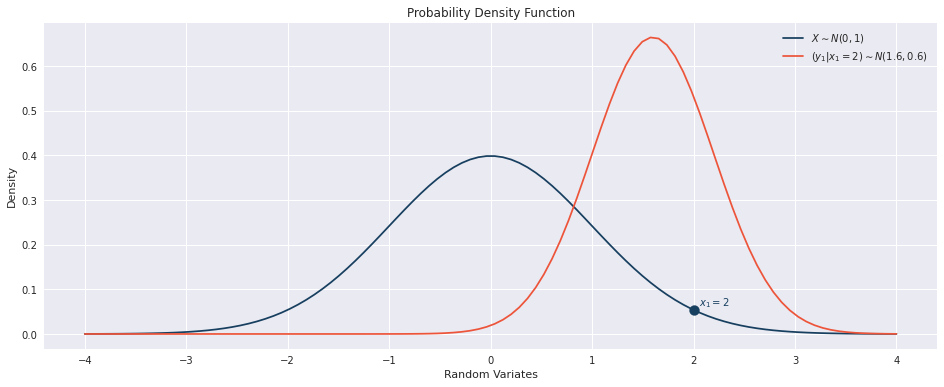
Example Simulation (\(x_1=2\))

Lets consider the example where \(X\) and \(Y\) are dependent Standard Normal distribution with a pearson correlation of \(\rho_{XY} = 0.8\) (i.e. they are 80% linearly correlation).

Lets also assume that we randomly sample \(x_1 = 2\) from \(X \sim N(0,1)\). Then the conditional distribution when selecting \(y_1\) is no longer a standard normal as shown below

Simulating Gaussian Copula

The process to calculate \(X\) and \(Y\) is as follows:

1. Obtain random variates \(Z_X, Z_Y \sim N(0,1)\) assuming indepences (\(\rho = 0\)). Sampling standard normal distributions as a starting point is why we define this as a Gaussian Copula.
2. Apply the Cholesky Decomposition to \(Z_X\) and \(Z_Y\) to get \(X, Y \sim N(0,1)\) such that they retain their linear dependence (\(\rho = 0.8\))

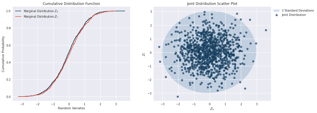
Step 1: Independent Random Variates

The first step is to simply simulate \(Z_X\) and \(Z_Y\) from two Standard Normal Distributions independently. The charts below show that the CDFs for each distribution are similar and that there is no dependence structure due to the symetric nature of the variance.

Step 2: Cholesky Decomposition and Determine \(X\) and \(Y\)

Once we have drawn our \(Z_X\) and \(Z_Y\) from independent Standard Normal distribution, we now have to take into account the dependence structure between the two samples by applying Cholesky Decomposion.

For a two-dimentional correlation matrix \(\rho\) defined as

The Cholesky Decomposition is

Therefore we can calculate \(X\) and \(Y\) as follows:

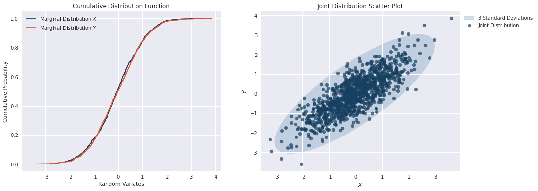
the results below show that the marginal distributions of \(X\) and \(Y\) look the same as \(Z_X\) and \(Z_Y\), however the joint distribution is clearly shows the dependence structure. This demonstrates an example as to why we do not nessassarily know the join distribution given the marginal distributions. The Copula is also needed to understand the joint distribution.

Python implementation

A code below demonstrates the implementation of the Gaussian copula in Python.

import scipy as sp
import numpy as np

def copula_gaussian(n, p, seed):
    
    ''' 
    n: Number of simulation
    p: Pearson's correlation coefficient
    seed: Random seed
    '''
    
    # Independed Normal distributions
    Z_x = sp.stats.norm.rvs(loc=0, scale=1, size=n, random_state=seed)
    Z_y = sp.stats.norm.rvs(loc=0, scale=1, size=n, random_state=seed*2)
    Z = np.matrix([Z_x, Z_y])
    
    # Construct the correlation matrix and Cholesky Decomposition
    rho = np.matrix([[1, p], [p, 1]])
    cholesky = np.linalg.cholesky(rho)
    
    # Apply Cholesky and extract X and Y
    Z_XY = cholesky * Z
    X = np.array(Z_XY[0,:]).flatten()
    Y = np.array(Z_XY[1,:]).flatten()
    
    # CDF
    X_cdf = sp.stats.norm.cdf(X, loc=0, scale=1)
    Y_cdf = sp.stats.norm.cdf(Y, loc=0, scale=1)
    
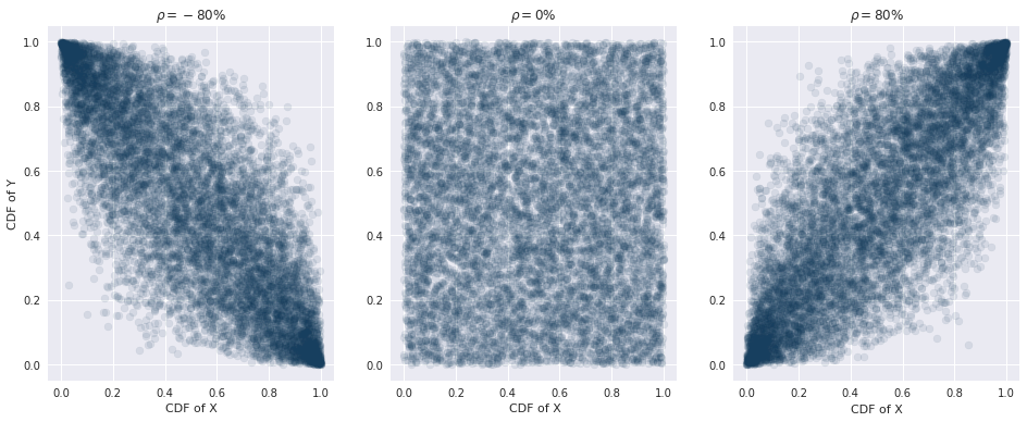
    return (X, Y, X_cdf, Y_cdf)

The chart belows shows the sensitivity of the Gaussian copula to changes in the correlation coefficient \(\rho\).

Summary

Within this article we discussed how we can determine a joint distribution from a set of marginal distributions by using a Gaussian copula. We also explained that Gaussian copulas are generally used when the distributions are not fat-tailed. In the case when our distributions are highly skewed and fat-tailed, then another choice of copula such as the t-copula may be more suitable. We also demonstrated an example of how we could simulate a Gaussian copula using Python.